Mastering Linear Inequalities in Two Variables: The Essential Answer Guide from Lesson 7 3

Unlocking the power of linear inequalities in two variables is a foundational challenge in algebra—one that shapes problem-solving across mathematics, science, and real-world applications. The Lesson 7 3 Answer Key presents a decisive framework that transforms abstract concepts into practical tools, revealing how to interpret, solve, and visualize these inequalities with precision. This article unpacks the core strategies, key principles, and common pitfalls from this pivotal lesson, providing a comprehensive roadmap for students, educators, and lifelong learners aiming to excel in algebra.

Core Concepts: What Are Linear Inequalities in Two Variables?

At their essence, linear inequalities in two variables define regions on the coordinate plane where a linear relationship satisfies an inequality—either “less than,” “greater than,” “less than or equal to,” or “greater than or equal to.” Unlike equations, which pinpoint exact solutions, inequalities describe infinite sets of solutions that lie within defined zones bounded by a straight line. The general form takes the type: ax + by ≤ c or ax + by > c, where *a*, *b*, and *c* are real numbers, and *x* and *y* represent variables. Understanding the direction of the inequality—determined by the inequality symbol—is crucial, as it governs which side of the boundary line represents valid solutions.

An essential diagnostic concept from Lesson 7 3 is recognizing that the inequality symbol informs how the terminal side of the boundary line is shaded in graphical representation. This visual shading, quantified through test points, reflects the true solution set across the plane. As textbooks emphasize: “A boundary line may be solid or dashed to indicate inclusion or exclusion of boundary points,” a distinction that directly affects how inequality solutions are interpreted and applied.

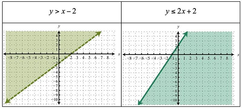
Graphical Representation: Drawing Solutions Step by Step

Translating an inequality into a graph requires a systematic approach, one refined through the Lesson 7 3 Answer Key. The process begins with identifying the boundary line, derived by turning the inequality into an equation. This line divides the plane into two half-planes, and the correct region must be determined based on inequality direction.

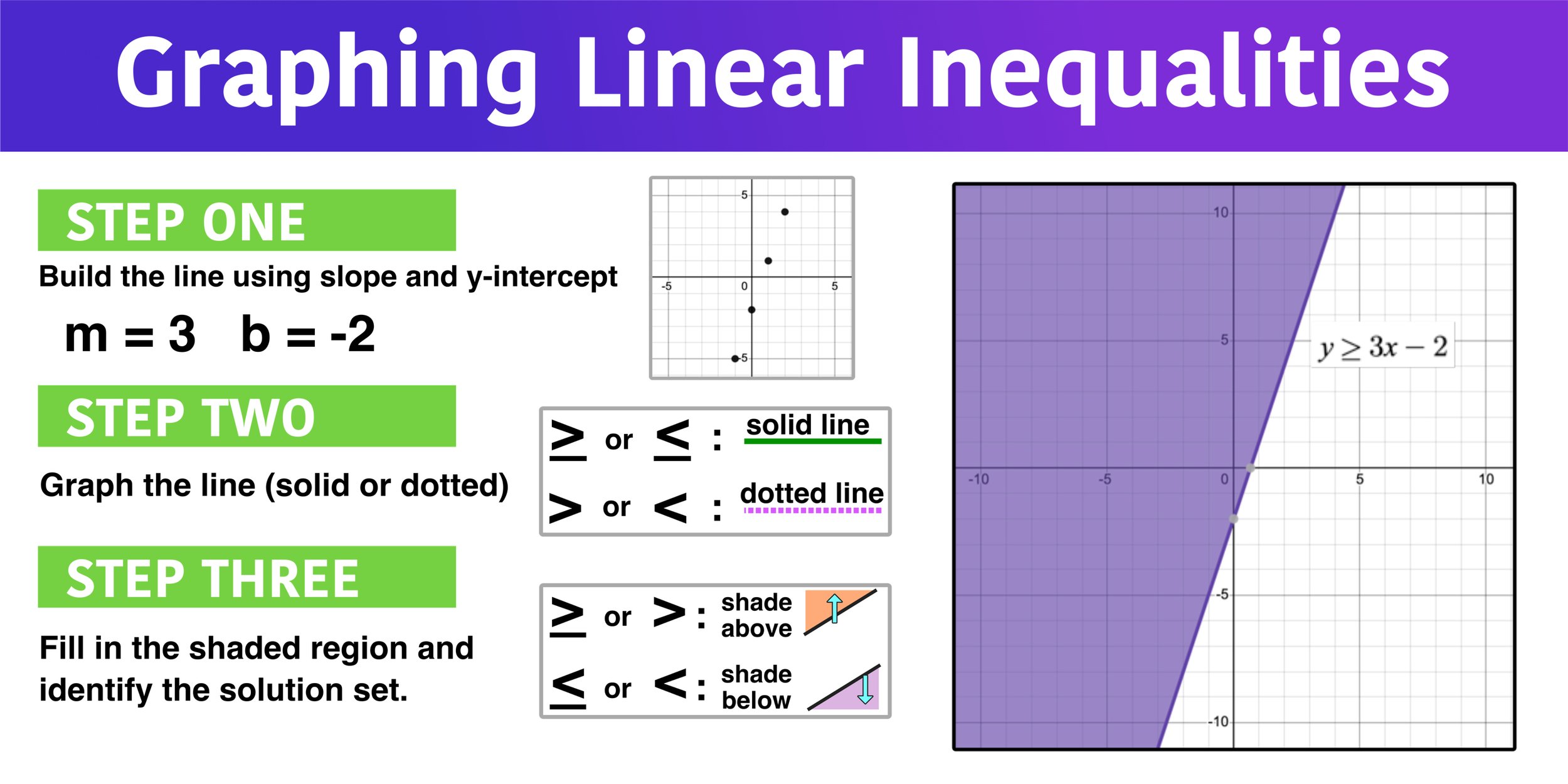
1. Convert the inequality to an equation and graph the boundary line first. Use a solid line if ≤ or ≥, and a dashed line if < or >.
2. Select a test point not on the line—typically (0,0) if not on the line—and substitute into the original inequality.
3. Evaluate whether the test point satisfies the inequality; shade the appropriate half-plane accordingly.
4. Verify edge points: if the inequality includes “≤” or “≥,” points on the boundary are included and shaded accordingly.

“Accuracy in identifying the shading direction is the linchpin between algebraic expression and geometric truth,” observes algebraic education specialist Dr. Elena Marquez in her analysis of inequality visualization.

The answer key emphasizes that visual correctness—not just solving—is central.

Misjudging shaded regions leads to flawed conclusions, especially in applications such as budget constraints, safety zones, or comparative evaluations.

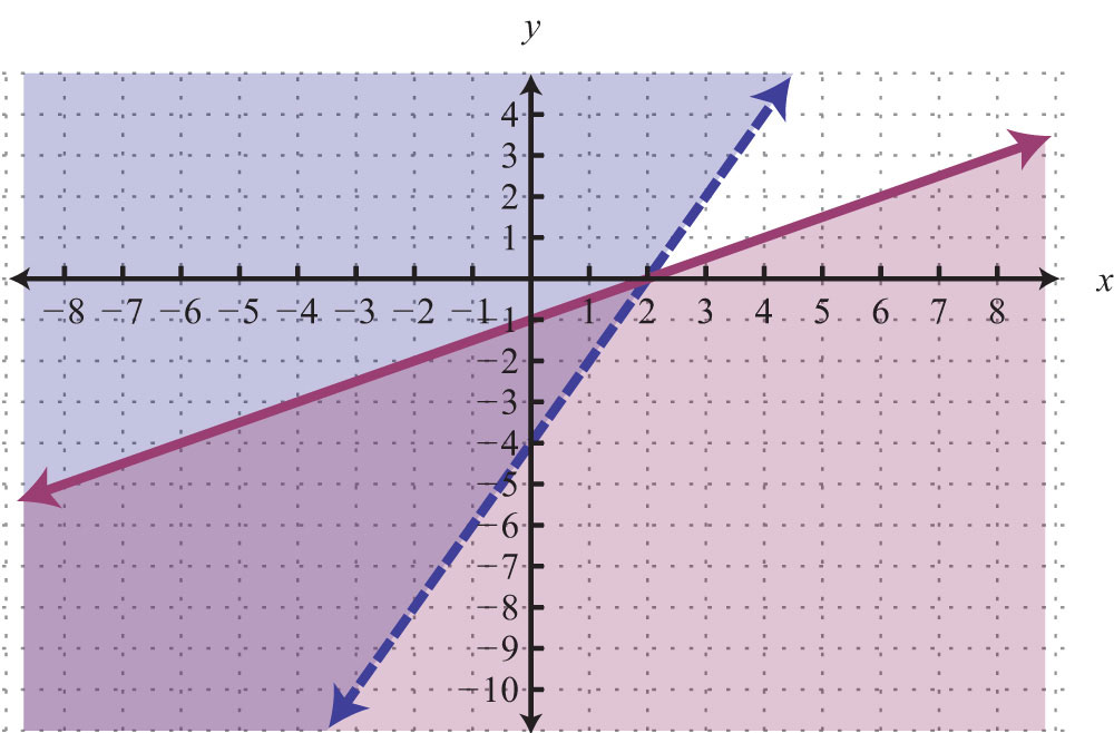
Critical Techniques: Solving Systems of Two Linear Inequalities

Beyond individual inequalities, the Lesson 7 3 Answer Key strengthens understanding through systems—setting up and solving multiple inequalities that intersect to define a shared solution region. This concept is vital in optimizing resources, mapping feasible zones in economics, or modeling multi-constraint scenarios in engineering.

Solving such systems hinges on recognizing overlapping solution sets. For example: x + y ≤ 6 2x − y ≥ 3 Suppose a manufacturer must allocate materials such that both constraints are met—units produced and labor hours remain within defined limits. Graphing each inequality reveals a bounded polygon: the vertices of which represent optimal production mixes.

Key strategies include: • Identifying the boundary lines for each inequality, • Determining the feasible region by testing quadrants or intersection points, • Using graphical methods or substitution/elimination for precise solution vectors, • Recognizing special cases such as parallel lines (no solution) or coinciding lines (infinite solutions). A common entry point for students is mapping each inequality to real-world variables: - *x* = hours worked - *y* = units produced - *x + y* = total output Then, solving concurrent inequalities uncovers viable operational plans that satisfy all constraints simultaneously.

Applications Beyond the Classroom: Real-World Relevance

One of the most compelling aspects of mastering linear inequalities in two variables is their broad applicability.

From economics—maximizing profit under resource limits—to environmental science—defining pollution thresholds—this mathematical framework translates abstract equations into actionable insights. For instance: - **Budgeting:** A business may use inequalities to stay under a monthly cost cap: *c₁x + c₂y ≤ B*, balancing product prices (*x*, *y*) against available funds (*B*). - **Logistics:** Delivery schedules often conform to time windows; inequalities model on-time arrival constraints.

- **Engineering Design:** Material usage and structural integrity must remain within tolerances expressed as linear limits. The Lesson 7 3 Answer Key reinforces that performance on graphical problems directly enhances data-driven decision-making, equipping learners to interpret not just equations, but the boundaries of possibility.

Common Pitfalls and How to Avoid Them

Despite its utility, learning linear inequalities presents recurring challenges.

The answer key serves not only as a guide to correctness but also as a warning against simple errors: - **Skipping the test point:** Relying on intuition without validation often leads to incorrect shading. Always confirm which half-plane satisfies the inequality. - **Misinterpreting the inequality symbol:** The phrase “greater than or equal to” demands inclusion of boundary points—ignoring this creates incomplete solutions.

- **Confusing overlapping systems with singular plots:** Systems require joint analysis; solving each pairwise neglects critical intersection logic. - **Neglecting to sketch before solving:** Visually mapping variables first prevents algebraically derived mistakes.

“It is not the problem that determines your approach, but your mastery of the tools—precision in graphing, clarity in logic,” advises algebra expert Dr.

Raj Patel.

Recognizing these frequent missteps enables learners to shift from mechanical solving to strategic understanding.

The Enduring Value of the Lesson 7 3 Answer Key

Mastering linear inequalities in two variables is more than an academic task—it is a gateway to analytical rigor. The Lesson 7 3 Answer Key distills complexity into clarity, transforming abstract algebraic expressions into visual, actionable models.

By emphasizing graphical accuracy, system solving, real-world relevance, and error prevention, it empowers learners to navigate mathematical uncertainty with confidence. As the inequality symbol itself whispers, “Where does this leave us?”—the answer lies not just in symbols, but in informed choice, structured thinking, and the quiet power of properly interpreted constraints. This foundation forms the backbone of advanced mathematics, equipping tomorrow’s thinkers with tools to solve not just problems, but the boundaries of possibility