Grafana Queries Made Easy: Decode Time-Series Data with Practical Examples

Unlock the power of time-series visualization with Grafana’s intuitive query language — no coding expertise required. Grafana thrives on its ability to transform raw metrics into actionable insights, and mastering basic query examples transforms complexity into clarity. Whether monitoring server performance, tracking application metrics, or analyzing IoT data streams, knowing how to shape queries empowers users at every level.

This guide distills the most effective Grafana query patterns into clear, real-world use cases, proving that effectively reading and writing queries is the key to unlocking Grafana’s full potential.

The Core Syntax: Postgres Queries Power Grafana

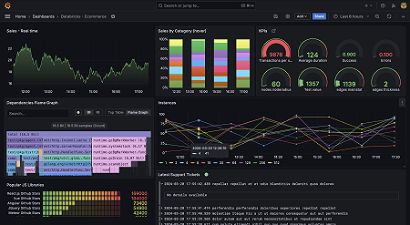
At foundation, Grafana relies on Postgres-style SQL-like queries embedded directly into dashboards. The core structure follows familiar SQL patterns — SELECT statements joined with WHERE, ORDER BY, and grouping clauses — but optimized for time-series data.

For example: ```sql SELECT metric_name, AVG(value) AS avg_value, count() AS total_samples FROM your_target_table WHERE time >= now() - INTERVAL '1h' GROUP BY metric_name, time_hour ORDER BY time_hour ``` This query retrieves hourly aggregates of critical metrics over the last hour, forming the backbone for performance monitoring and anomaly detection. By constraining data with time intervals and grouping by time buckets, analysts can distill hours of raw data into compact, meaningful summaries. Grafana automatically parses these queries, rendering responsive time panels, heatmaps, and statistical cards that update in real time.

Understanding these fundamentals transforms how data is interpreted—not just seen.

Mastering Time-Series Filtering: The Crucial WHERE Clause

Time is the lifeblood of monitoring, making precise temporal filtering nonnegotiable. Crucial queries begin with filtering data by time ranges—a function available exclusively in Grafana’s query language: `WHERE time >= ` and `WHERE time < `.

Using `now()` gives the current moment, while `ago()` expresses relative durations: `ago(24h)` captures the last day. David Brooks of Grafana Labs emphasizes, “Time-based filtering is where Grafana shifts raw data into context.” For instance, tracking recent error rates in a web application requires filtering: ```sql SELECT status, COUNT(*) AS error_count FROM logs WHERE time >= now() - interval '12h' AND status = 'error' GROUP BY status, time_hour ORDER BY error_count DESC ``` This query isolates critical error occurrences over the past 12 hours, enabling rapid root cause investigations. Without accurate time scoping, even the most detailed metrics become noise.

Aggregation Patterns: Summarizing at Scale

Raw metrics alone rarely reveal trends — aggregation turns them into narratives. Common functions include `AVG()`, `SUM()`, `MAX()`, `MIN()`, and `STDEV()` for variance. These aggregations work in tandem with time intervals to surface patterns: spikes, averages, and deviations.

A typical operational metric might aggregate every 5 minutes into hourly averages: ```sql SELECT metric_name, AVG(value) AS avg_reading, MAX(value) AS peak, MIN(value) AS trough FROM sensor_readings WHERE time > now() - interval '2h' GROUP BY metric_name, time_hour ``` This structure enables observability teams to detect shifts in system behavior, spot performance degradation, or celebrate uptime stability. Combined with Grafana’s built-in visualization engine, such queries render trend lines that evolve live, turning abstract numbers into stories of reliability. Another powerful example compares average server response times across regions: ```sql SELECT region, AVG(response_time_ms) AS avg_response, PERCENTILE_CONT(0.75) WITHIN GROUP (ORDER BY response_time_ms) AS p75 FROM api_latencies WHERE region IN ('us-east', 'eu-west') GROUP BY region ORDER BY avg_response ``` Here, percentile aggregation identifies thresholds beyond normal performance, spotlighting regional discrepancies that demand attention.

Dynamic Filters and Dashboard Interactivity

Grafana’s strength lies not in static displays but in responsive, user-driven dashboards. Dynamic filters leverage variable substitution to enable interactive exploration. By defining filters as variables—such as time ranges, service labels, or environment tags—users can instantly refresh visualizations based on selection.

Consider a filtering example using an input field: ```sql WITH selected_env AS "${variables.env}", SELECT metric_name, IF(time >= now() - interval selected_env.hours_ago, avg(cpu_usage), NULL) AS cpu_usage FROM system_metrics WHERE env = selected_env ORDER BY time DESC LIMIT 10 ``` This query, embedded in a dashboard panel with a time slide or dropdown, allows analysts to instantly compare metrics across environments. The `IF()` function safely returns NULL outside the filtered range, avoiding misleading empty cells. Interactive filtering transforms panels from passive displays into insight engines that adapt to user intent, accelerating decision cycles.

Such interactivity aligns with modern expectations of data engagement—where dashboards respond, refine, and reveal with minimal friction.

Structured Query Examples for Real-World Use Cases

From infrastructure monitoring to microservices observability, standardized Grafana queries solve recurring challenges. Below are practical examples drawn from enterprise deployments.

**1. Monitoring Application Error Rates Tracking service health through error tracking is critical. Grafana’s SQL supports multi-step filtering and conditional formatting: ```sql SELECT status, COUNT(*) AS error_count, rate(response_time_ms_500{status='error'}) / count(*) AS error_rate_percent FROM requests WHERE status = 'error' AND time >= now() - interval '1h' GROUP BY status, time_hour ORDER BY error_count DESC ``` This query calculates both error count and rate (as a percentage of total requests), offering a normalized view beyond absolute numbers.

The `rate()` function normalizes spikes over time, making short-lived surges distinguishable from sustained issues. **2. Trend Analysis of Resource Utilization Evaluating CPU and memory trends reveals capacity needs and optimization opportunities: ```sql SELECT time_bucket('1h', time) AS bucketed_time, avg(cpu_usage_percent) AS cpu_avg, avg(memory_usage_mb) AS memory_usage FROM system_cpu_memory